Table Engines

The table engine determines the way data is organized and stored, the method and type of indexing, which queries are supported, and how they are supported, as well as some other specific features and configurations. In ByConity, the most commonly used table engines are CnchMergeTree, CnchKafka, and CnchMaterializedMySql. This article focuses on explaining the principles of these three table engines.

CnchMergeTree Table Engine

Implementation Principles

The CnchMergeTree table is the most commonly used table engine. Its core concept is similar to LSM-Tree. Data is partitioned based on the partition key (partition by) and then sorted and stored based on the sorting key (order by). Key features include:

• Logical Partitioning (Partition): If a partition key is specified, data is divided into different logical datasets (logical partitions, Partition) based on the partition key. Each logical partition can contain zero or multiple data parts (DataPart). If the query conditions can be used to prune partitions, it usually speeds up the query. If no partition key is specified, all data is stored in a single logical partition.
• Data Parts (Fragment): Data within a data part is sorted based on the sorting key. Each data part also has a min/max index to accelerate partition selection.
• Data Granules (Granule): Each data part is logically divided into granules. The default granule size is 8192 rows (determined by the table's index_granularity configuration). Granules are the smallest indivisible data sets for data queries in ByConity. The first row of each granule is marked by the primary key value of that row. ByConity creates an index file for each data part to store these markers. For each column, regardless of whether it is included in the primary key, ByConity stores similar markers. These markers allow you to directly find data in the column files. As the target of ByConity's sparse index, granules are also the smallest units for data scanning in memory.
• Background Merging: Background tasks periodically merge DataParts within the same partition while maintaining the sorting order based on the sorting key. Background merging reduces the number of Parts for more efficient storage and improved query performance.

Table Creation Statement and Related Configurations

CREATE TABLE [IF NOT EXISTS] [db.]table_name
(
    name1 [type1] [NULL|NOT NULL] [DEFAULT|ALIAS expr1] [compression_codec] [TTL expr1],
    name2 [type2] [NULL|NOT NULL] [DEFAULT|ALIAS expr2] [compression_codec] [TTL expr2],
    ...
    INDEX index_name1 expr1 TYPE type1(...) GRANULARITY value1,
    INDEX index_name2 expr2 TYPE type2(...) GRANULARITY value2,
) ENGINE = CnchMergeTree()
ORDER BY expr
[PARTITION BY expr]
[CLUSTER BY (column, expression, ...) INTO value1 BUCKETS SPLIT_NUMBER value2 WITH_RANGE]
[PRIMARY KEY expr]
[UNIQUE KEY expr]
[SAMPLE BY expr]
[TTL expr]
[SETTINGS name=value, ...]

Designing the Partition Key (PARTITION BY)

The partition key defines partitions, which are logical datasets divided within a table based on specified rules. You can partition by any criterion, such as date. To minimize the amount of data that needs to be operated on, each partition is stored separately. During queries, ByConity tries to use the smallest subset of these partitions. The partition key is specified using the PARTITION BY expr clause when creating the table. The partition key can be any expression involving columns in the table. For example, to partition by month, the expression would be toYYYYMM(date). Alternatively, you can use an expression tuple like (toMonday(date), EventType).

It's important to note that the range of values calculated by the partition expression in the table should not be too large (recommended to be no more than 10,000). Having too many partitions can consume significant memory and lead to increased IO and computational overhead.

Properly designing the partition key can significantly reduce the amount of data that needs to be scanned during queries. Generally, it's recommended to design the partition key based on the most commonly used conditions in queries, while ensuring that the range of values does not exceed 10,000 (such as date).

Designing the Sorting Key (ORDER BY)

The sorting key can be a tuple of columns or any expression. For example: ORDER BY (OrderID, Date). If no sorting is required, you can use ORDER BY tuple(). Data within a DataPart is sorted based on the sorting key. Please note that the fields used in the order by clause cannot be modified after the table is created.

Designing the Primary Key (PRIMARY KEY)

By default, there is no need to explicitly specify the primary key. ByConity uses the sorting key as the primary key. However, in special scenarios where the primary key and sorting key differ, the primary key must be the leftmost prefix of the sorting key. For example, if the sorting key is (OrderID, Date), the primary key must be OrderID and cannot be Date. In some special table engines, such as CnchAggregatingMergeTree and CnchSummingMergeTree, the primary key may differ from the sorting key.

ByConity creates a sparse index on the primary key, with granules as the unit (in contrast to a dense index, which creates index information for every row). If the query conditions match the leftmost prefix of the primary key index, the primary key index can quickly filter out the granules that may need to be read, which is typically much more efficient than scanning the entire DataPart.

Additionally, it's important to note that the PRIMARY KEY does not guarantee uniqueness, so it's possible to insert rows with duplicate primary keys. Partitioning (PARTITION BY) and the primary key (PRIMARY KEY) are two different ways to accelerate data queries. When defining them, it's generally recommended to use different columns to cover more query scenarios. For example, avoid repeating the first column of the order by clause in the partition by clause. Here are some considerations for choosing the primary key:

• Whether it is a commonly used column in query conditions.
• Avoid using the first column that is not the partition key.
• Consider the selectivity of the column. For example, columns with few distinct values (such as gender or yes/no) are not recommended for inclusion in the primary key.
• If the current primary key is (a, b) and the data range covered by (a, b) is large (spanning multiple granules), consider appending a new commonly used query column to the primary key to filter more data.
• Longer primary keys can negatively impact insertion performance and memory consumption but have no impact on query performance.

Designing the Unique Key (UNIQUE KEY)

The primary key (PRIMARY KEY) does not guarantee deduplication. If there is a need for unique key deduplication, a unique key index must be set when creating the table. After setting the unique key, ByConity provides an upsert update semantics, allowing efficient updating of data rows based on the unique key. Queries automatically return the latest value for each unique key.

The unique key can be a tuple of columns or any expression, such as UNIQUE KEY (product_id, sipHash64(city)). Unique key indexing can be controlled by configuring partition_level_unique_keys to determine whether it is unique at the partition level or across the entire table. Currently, it is recommended to use partition-level unique keys with no more than 10 million rows per partition. If unique keys are set at the table level, it is recommended to have no more than 10 million rows in the entire table.

When querying using a unique key, the unique key index is used to filter data and accelerate the query. Therefore, the primary key can typically be set to different columns than the unique key to cover more query conditions. However, if partial column updates are required, the unique key must be the leftmost prefix of the sorting key.

• Related Configurations:
  • partition_level_unique_keys: Determines whether the unique index is at the partition level. The default value is true. If set to false, the unique index applies to the entire table.
  • cloud_enable_staging_area: Determines whether asynchronous write mode is enabled. The default value is false.

Index (Skip Index)

When creating a table, a skip index can be defined as follows:

INDEX index_name expr TYPE type(...) GRANULARITY granularity_value

• Available index types: minmax stores the extreme values of the specified expression (if the expression is a tuple, it stores the extreme values of each element in the tuple). This information is used to skip data blocks, similar to a primary key. The skip index feature is currently in testing, and supported skip index types will be added once completed.

Granule Configuration

• index_granularity - Index granularity. The number of data rows between adjacent 'marks' in the index (corresponding to Granule size). The default value is 8192.

The following three configurations are pending testing and have not been verified by RD for functionality.

• index_granularity_bytes - Index granularity in bytes, with a default value of 10Mb. If you want to limit the index granularity only by the number of data rows, set it to 0 (not recommended).
• min_index_granularity_bytes - The allowed minimum data granularity, with a default value of 1024b. This option is used to prevent misoperations, such as adding a table with a very low index granularity.
• enable_mixed_granularity_parts - Whether to enable controlling index granularity size through index_granularity_bytes. In older versions, only the index_granularity configuration could be used to limit the index granularity size. When querying data from tables with very large rows (tens or hundreds of megabytes), the index_granularity_bytes configuration can improve ByConity performance. If your table has very large rows, you can enable this configuration to improve the performance of SELECT queries.

TTL for Columns and Tables

Specifies the duration for storing rows and defines a list of rules for moving data fragments on hard drives and volumes. This is an optional feature.

At least one column of type Date or DateTime must be present in the expression, for example:

TTL date + INTERVAl 1 DAY

For more details, please refer to TTL for Tables and Columns

Best Practices

• Best practices for primary key indexes:

https://clickhouse.com/docs/zh/guides/improving-query-performance/sparse-primary-indexes/

• Best practices for secondary indexes:

https://clickhouse.com/docs/zh/guides/improving-query-performance/skipping-indexes

• Column type considerations:

Avoid blindly using the String type.

If possible, use Int(8|16|32|64|128|256) / Date / Date32 / DateTime / DateTime64 / Float / Decimal instead of String.

A simple way to determine this is to check if the conversion to the target type is possible, such as SELECT countIf(toUInt8OrNull(col) IS NULL) FROM table, SELECT countIf(toDateOrNull(col) IS NULL) FROM table.

For String columns with relatively fixed content, consider using Enum instead, such as province names. Enum values can be added later through ALTER TABLE.

Use FixedString if the minimum and maximum lengths of the String do not differ by more than 8, as String requires an additional 8 bytes of offset storage compared to FixedString in memory: SELECT min(length(col)), max(length(col)) FROM table.

• Nullable selection:

If you are certain that the column does not contain Null values, avoid using the Nullable type as it can negatively impact performance.

• LowCardinality:

If a column has a low cardinality, meaning there are no more than 10,000 distinct values within a DataPart, consider using the LowCardinality type. The LowCardinality type applies dictionary encoding to the original column. For many applications, processing dictionary-encoded data can significantly increase query speed, reduce storage space, and improve IO efficiency.

• Reference documentation:

https://clickhouse.com/docs/zh/engines/table-engines/mergetree-family/mergetree#tiao-shu-suo-yin-fen-duan-hui-zong-suo-yin-shi-yan-xing-de

https://clickhouse.com/docs/en/sql-reference/statements/create/table/#column-compression-codecs

CnchKafka Table Engine

Functional Definition

CnchKafka is a table engine developed by ByConity based on the community's ClickHouse Kafka table engine, specifically designed for the cloud-native architecture. It efficiently and rapidly ingests user data from Apache Kafka into ByConity. Its design and implementation not only adapt to the new cloud-native architecture but also enhance some functionalities compared to the community implementation.

Key features of CnchKafka include:

• Automatic fault tolerance based on cloud-native architecture advantages, reducing operational and maintenance costs.
• Scalable consumption capacity: Supports adjusting the number of consumers through SYSTEM commands, with a maximum adaptation to the number of partitions corresponding to the topic.
• Enhanced consumption semantics: Relies on Transaction guarantees and manages offsets through the engine to achieve Exactly-Once consumption semantics.
• Consumption performance: Heavily dependent on the schema complexity of the user table, with typical values ranging from 2k to 2M rows per second and a throughput of around 15MiB/s.
• Supports various data types, including but not limited to Json, ProtoBuf, CSV, etc.
• Supports recording consumption logs, facilitating problem troubleshooting and providing data audit capabilities.

Implementation Principles

CnchKafka inherits the basic design of the community, utilizing a triplet of <CnchKafka consumption table, Materialized View, and storage table> to achieve the entire consumption pipeline. Specifically:

• CnchKafka consumption table: Responsible for subscribing to Kafka topics and consuming messages; parsing the received messages into Blocks.
• Materialized View: Establishes a data pathway from the consumption table to the storage table, writes Blocks consumed by CnchKafka into the storage table, and provides simple filtering capabilities.
• Storage table: Supports various ByConity MergeTree storage tables.

The basic data pathway is as follows:

Architecture Diagram of CnchKafka Component in ByConity

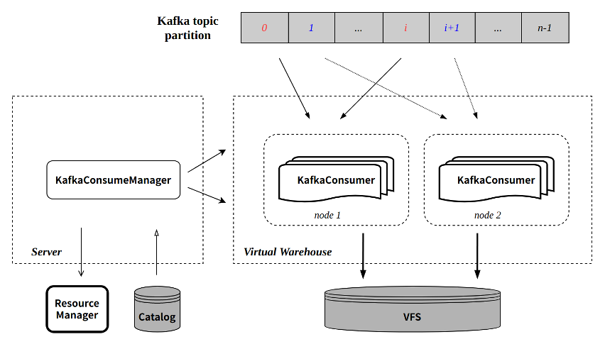
Component Description

Server

The application access layer serves as the entry point for all queries and import tasks. Designed as lightweight, it focuses on task scheduling, forwarding, and metadata access rather than executing specific queries or imports. Its responsibilities include:

• Preprocessing query requests by reading metadata from the Catalog, forwarding the raw data and query SQL to query nodes, and returning the query results to upper layers (APIs, users, etc.).
• Managing import tasks by selecting import nodes for task execution.
• Interacting with the Catalog to query or update metadata.
• Interacting with the Resource Manager to select task execution nodes for load balancing.

Virtual WareHouse

• The computing layer executes all query and import tasks as stateless services.
• Supports tenant isolation for resource and data separation.
• Enables read-write splitting, allowing queries and imports to create and specify different Virtual Warehouses.

Catalog

• A key-value database managing metadata, including database table metadata, partition metadata, etc.
• Also stores consumption offsets for CnchKafka.

VFS

• The underlying storage supports multiple storage systems, including HDFS, S3, etc.

KafkaConsumeManager

Each CnchKafka consumption table initiates a Manager at the Server layer responsible for scheduling and managing all consumer tasks. The Manager runs as a permanent thread on the Server, ensuring service stability through Server high availability and DaemonManager. The main functions of KafkaConsumeManager include:

• Evenly distributing topic partitions among consumers based on the configured number of consumers.
• Interacting with the Catalog to obtain partition consumption offsets.
• Scheduling consumers to execute on configured Virtual Warehouse nodes, supporting various strategies for node selection and load balancing.
• Regularly checking the liveliness of each consumer task to ensure stable task execution.

KafkaConsumer

Each KafkaConsumer runs as a permanent thread on a Virtual Warehouse node, consuming data from the specified topic partition, converting it into partitions written to the VFS, and submitting metadata back to the Server to be written to the Catalog. Key features include:

• Inherits the community's batch write mode (default consumption cycle of 8 seconds).
• Ensures atomicity through transactions during each consumption process: creates transactions through RPC interactions with the Server; transaction commits simultaneously submit written partition metadata and the latest consumption offset.

Exactly-Once

Compared to community implementations, CnchKafka enhances consumption semantics from At-Least-Once to Exactly-Once. This is primarily achieved through transaction guarantees provided by the new architecture. Each consumption round is managed transactionally, and each data metadata submission is accompanied by the corresponding offset. Since transactions ensure atomicity, either both the data metadata and offset are successfully submitted, or both fail. This ensures consistent data and offsets, allowing consumption to resume from the last submitted offset after each restart, achieving Exactly-Once semantics.

Automatic Fault Tolerance

CnchKafka employs a fast-fail strategy for fault tolerance:

• KafkaConsumeManager regularly checks the liveliness of consumer tasks. If a task fails, a new consumer is immediately started.
• During each execution, KafkaConsumer interacts with the Server through RPCs (creating and committing transactions) and validates its own validity with the Manager. If validation fails (e.g., if the Manager has already started a new consumer), the KafkaConsumer proactively terminates itself.

Designing Bucket Tables

Bucket tables are an optional table-level setting. When properly configured, the system organizes table data based on the user-provided Cluster Key (one or more columns or expressions from the table creation statement). Data with the same Cluster Key values is clustered under the same bucket number.

Clustering data using the Cluster Key can provide several benefits for large tables:

• Point queries on the Cluster Key can filter out most data, reducing IO and resulting in faster execution times and higher concurrent QPS.
• Aggregation queries on the Cluster Key can consume less memory and execute faster, further optimized with distributed_perfect_shard.
• Join operations on multiple tables using the Cluster Key can leverage co-located joins, significantly reducing shuffle data volume and execution time.

Due to the complexity of Bucket table settings, they are typically suitable for two scenarios:

• Large tables, where the number of partitions significantly exceeds the number of workers.
• Queries that can benefit from the aforementioned advantages.

Selecting the Cluster Key

The Cluster Key can consist of one or more columns or expressions, but it's recommended to use no more than three fields to avoid excessive write overhead and limit the scope of beneficial queries.

Choosing the right Cluster Key is crucial for performance and requires careful consideration. General guidelines include:

• Columns frequently used for equality or IN filters.
• Columns commonly used for aggregations.
• Join keys for multiple tables.

If a common scenario involves combining two columns (e.g., a = 1 and b = 2), using both as the Cluster Key can yield better results.

Another factor to consider is the number of distinct values for each column. Since data with the same Cluster Key values is grouped under the same bucket number, and all partitions under a bucket number are sent to the same worker for computation, it's important to:

• Have enough distinct values to utilize all worker nodes. The number of distinct values should ideally exceed the number of workers.
• If the number of distinct values is small, prefer columns with the highest distinct value count, ideally a multiple of the number of workers, to achieve more balanced data distribution during queries.

For example:

1. Consider a table named "test" with columns c1, c2, and c3, which are independent.
2. Assume there are 30 worker nodes.
3. The distinct count for c1 is 6.
4. The distinct count for c2 is 8.
5. The distinct count for c3 is 5.

In this case, none of the individual distinct counts meets the worker node count. While the combination of c1 and c2 has a distinct count of 48 (higher than the worker count), it's not an ideal Cluster Key since it's not a multiple of the worker count. However, combining c1, c2, and c3 results in a distinct count that is 8 times the worker count, providing a more balanced data distribution.

Selecting the Bucket Number

Within a partition:

• Each row is assigned a bucket number based on the Cluster Key value using the modulo operation (% BUCKETS).
• Partitions with the same bucket number are sent to the same worker node for computation.

Choosing an appropriate bucket number is crucial for both storage and query performance. General guidelines include:

• Ensure the bucket number is a multiple of the worker count to ensure balanced query distribution. It's typically recommended to set it as 1 or 2 times the worker count (to allow for future worker expansion).
• Ensure each bucket number within a partition has enough data to avoid generating excessively small partitions. For smaller tables, aim for at least 1GB of data per bucket number per partition. Avoid setting an excessively high bucket number, as it can result in having fewer bucket numbers than worker nodes.

Deciding on Cluster By Definition Changes

Over time, data changes, query patterns evolve, and the number of worker nodes may fluctuate. This might necessitate updating the Cluster Key or bucket number. However, making such changes comes with a cost and requires careful consideration:

• Modifying the Cluster Key necessitates reclustering existing data, which can be time-consuming depending on the data size.
• During the reclustering process, queries on the existing data revert to treating the table as a regular table, temporarily losing all Bucket table benefits.
• Reclustering consumes resources on the write workers, potentially impacting existing queries, merges, and other tasks. Therefore, it's essential to assess the current workload on the Cnch cluster and determine the optimal time for making such changes.

Two scenarios for modifying the Cluster By definition are:

• Changing the Cluster Key: This indicates that the current data arrangement no longer provides Bucket table benefits. Thus, there's no need to consider the temporary loss of benefits during reclustering. However, it's essential to evaluate the impact of the reclustering task on existing workloads to determine if and when it can be executed.
• Changing the bucket number: In this case, the current Bucket table benefits are still valuable. Therefore, it's crucial to coordinate with the business team to identify an acceptable performance degradation window and assess the duration of the reclustering process to determine the best time to proceed. Additionally, consider the impact of the reclustering task on existing workloads.